There are many people for whom calculating percentages is an uphill climb. And it is that despite being a simple operation, it is common to see errors in the formulas to calculate them. I won’t name names, but I have come across errors of this type even on professional websites, which are supposed to help people who have problems with them. I know that may sound excessive, but I guarantee you it’s true.
The luck is that, once again, we have the help of Excel, that application that is used for almost everything and that many of us find essential on a day-to-day basis. And yes, it is true that there are many operations that can be carried out with a normal calculator, such as the one included in Windows or those found on our smartphones (and calculating a percentage is among them), but why not go a little further? We are going to see three common operations related to percentagesand to create a spreadsheet that allows us to calculate them automatically.
Calculate the percentage of a number
This is obviously the simplest of these three calculators. What we are looking for with it is to enter a total and a percentage of it, and for the calculator to return the numerical value. Perhaps it is better understood with an example: if I enter 200 as a total, and 5% as a percentage, the calculator will return a 10, since 10 is 5% of 200.
We will start with the visual design of the calculator. In my case I like to differentiate, by means of colors, in which cells we must enter data and in which not. We can also block the cells in which the formulas will be included so as not to delete them by mistake, in another practical we will tell you how to do it. In any case, after applying formats and such, my calculator looks like this:
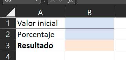
As you can deduce, we will have to enter the total in B1 and the percentage in B2. Remember, however, to apply the appropriate formats to these cells, that is, number to B1 and B3 and percentage to B2:
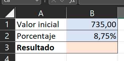
Now you just have to go to B3 and write the following formula: “=B1*B2” (without the quotes). And that’s it. With that simple formula you will already have the basic percentage calculator:
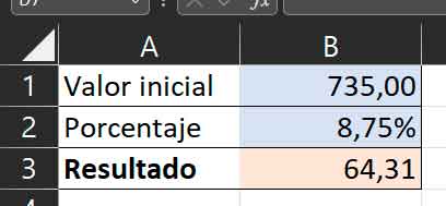
Remember, yes, change the references to the cells if you use other than those shown in the images.
Calculate the percentage value of one number with respect to another
Let’s turn the situation around. Imagine that what you want is to indicate two figures and that the calculator tells you what is the percentage value of B with respect to A. Again with an example, that if you indicate that A is 200 and that B is 80, the calculator tells you that 80 is 40% of 200.
As with the previous one, carry out the visual design of it, in my case it is the following:
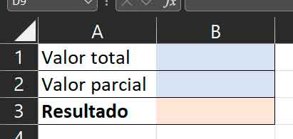
Of course, in this case you will have to apply number format to cells B1 and B2, and percentage to B3. With all this ready, go to B3 and write the formula “=1/B1*B2” (again, of course, without the quotes) and the calculator will be ready:
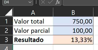
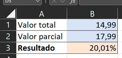
Note that in the example the value of B is lower than the value of A, but in reality it can also be used in reverse, for example to calculate the percentage value of a price increase. For this purpose you can keep in mind that you must subtract 100 from the result, or you can use this modified version of the formula: “=(1/B1*B2)-1”.
Break down the part of VAT in a price
Imagine that you have paid for a product or service and you only know the final amount that you had to pay, but not how much of it corresponds to VAT. The good news is that if you know what rate has been applied, calculating it is very easy. Let us remember that, in Spain, these are the three types of VAT:
| VAT rate | Tax rate |
| General | 21.00% |
| Reduced | 10.00% |
| super reduced | 4.00% |
And what we want is a calculator to provide the final price that we have paid and the corresponding VAT rate, and that in response gives us what we have paid as a rate and the amount without VAT. In this case, therefore, we will use two input fields and two output fields, something like this:
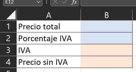
In this case we will apply the currency format to cells B1, B3 and B4 and the percentage format to cell B2. With everything ready, we will type the formula “=(B1/(1+B2))*B2” in cell B3, and then “=B1-B3” in cell B4. Thus, when we enter the corresponding values in B1 and B2, we can see the VAT breakdown:
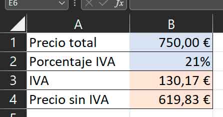
As you can see, performing this type of operation is really easy with Excel. And if you want to see more Microsoft spreadsheet tricks, here you can find another three that can be very practical for you.


